
 |
Linear and Nonlinear Inverse Problems with Practical ApplicationsJennifer L. Mueller and Samuli Siltanen |
EIT with the D-bar Method: Smooth and Radial Case
This page contains the computational Matlab files related to the book, which you can purchase in the SIAM Bookstore.
This page is related to a smooth and rotationally symmetric conductivity.
Introduction
The D-bar method is a reconstruction method for the nonlinear inverse conductivity problem arising from Electrical Impedance Tomography. This page contains Matlab routines implementing the D-bar method for a smooth and rotationally symmetric conductivity.
Note carefully that although we use the rotational symmetry of the conductivity to speed up some computations, the reconstruction process including the solution of the D-bar equation is two-dimensional, not one-dimensional.
Please download the Matlab routines below to your working directory and run them in the order they appear.
Definition of the example
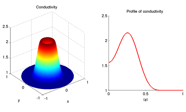
The first example concerns a rotationally symmetric and smooth conductivity that equals one near the unit circle. Outside the unit disc the conductivity has value 1.
The following file defines a rotationally symmetric and smooth conductivity in the unit disc: sigma.m.
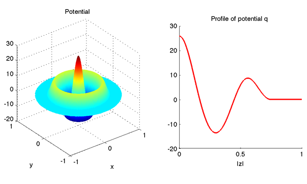
Furthermore, this file implements the Schrödinger potential related to the conductivity: poten.m.
The Laplace operator appearing in the definition of the potential is implemented by finite differences in poten.m. The following routines plot the conductivity and the potential, respectively:
Please run the plot commands before continuing to make sure that everything is working properly. You should see something like this:
Computation of the scattering transform via the Lippmann-Schwinger equation
Next we define a set of points in the k-plane for evaluating the scattering transform t(k).
Because of the rotational symmetry of this example, it is enough to choose k-values along the positive real axis: the scattering transform is known in this case to be rotationally symmetric and real-valued. Why? See proof.
So please download and run this file: kvec_comp.m.
The above file kvec_comp.m defines a set of k-points and saves them to a file called 'data/kvec.mat'. (Note that kvec_comp.m creates a subdirectory called 'data'. If you already created it before, Matlab will show a warning. However, you don't need to care about the warning.)
When running the example for the first time you might just use the file kvec_comp.m as it is. Later you might want to modify it to choose a different set of k-values.
Now that we have decided on the k-points, it's time to evaluate the scattering transform. Here we do it first by 'cheating', or by knowing the actual conductivity, because then there are no ill-posed steps involved. Later we will compute the scattering transform also honestly from (simulated) EIT measurements. This is the file that evaluates the scattering transform t(k) at the k-points: tLS_comp.m.
The result will be saved to a file called 'data/tLS.mat'. Here 'LS' refers to the use of the Lippmann-Schwinger equation in the computation of the complex geometric optics solutions. tLS_comp.m needs these files:
green_faddeev.m
g1.m
GV_grids.m
GV_LS.m
GVLS_solve.m
GV_project.m
GV_prolong.m
In the names of the above files, 'GV' refers to Gennadi Vainikko, a numerical analyst who invented the periodization-based algorithm used here for solving Lippmann-Schwinger type equations.
It is interesting to compare the linear and nonlinear Fourier transform. To that end, we compute the Fourier transform of the potential q using the routines Fq_comp.m and gaussint.m.
After running the files tLS_comp.m and Fq_comp.m, you can plot the results using tLS_plot.m.
You should see something like this:
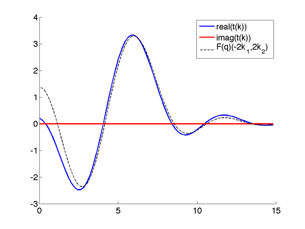
In the above image, the scattering transform is not quite approaching the value t(0)=0 as k tends to zero, although we know from theoretical results that this should be the case. Why such an error at zero? This is because we only used the value M=7 for constructing the grid, which was then of size 128x128. The Faddeev fundamental solution has a log(|k|) singularity at the origin, and the Lippmann-Schwinger type approach has always difficulties near the origin. You can either use as big M value as your patience and computer memory allows, or you can use the boundary integral equation approach below to compute t(k) for k near zero.
The rule of thumb is: The Lippmann-Schwinger approach for computing t(k) is good for k somewhat away from the origin, and the boundary integral approach for computing t(k) is good (only) for k near zero.
Simulation of EIT data
Since the conductivity is rotationally symmetric, the Dirichlet-to-Neumann map can be approximated by a diagonal matrix in the Fourier basis. Why? See proof.
The diagonal elements have been precomputed and are simply given as a data file DN1eigs.mat.
The DN matrix is constructed by the routine DN_comp.m.
For details of the computation of the matrix elements, see Mueller J L and Siltanen S 2003, Direct reconstructions of conductivities from boundary measurements, SIAM Journal of Scientific Computation 24(4), pp. 1232-1266. PDF (617 KB)
Computation of the scattering transform via the boundary integral equation
We need to build matrices for the single layer operators S_k parametrized by the complex number k. This is done by the routines Hk_comp.m and H1.m.
Here Hk_comp.m computes the matrices and H1.m is an auxiliary function. Note that the order Ntrig of trigonometric approximation (in other words, the number of basis functions used) has been chosen in the routine DN_comp.m above and saved to disc for later reference. The routine Hk_comp.m loads Ntrig from file.
Running the routine Hk_comp.m is computationally the most demanding task on this page. Do not be surprised if it takes 10 minutes or more.
Note that we save time by not running Hk_comp.m for too large values of |k|. Namely, the ill-posedness of the EIT problem has the effect that the boundary integral equation cannot be solved for |k| exceeding a certain threshold value R; for k values satisfying |k|>R the computation will produce numerical garbage.
Once Hk_comp.m has been run, we can solve the boundary integral equation for the traces of the complex geometric optics solutions. This is done by the routine psi_BIE_comp.m, and the result is saved to a file in the subdirectory 'data'. The next step is to evaluate the scattering transform by integration over the boundary using the routine tBIE_comp.m.
We are now ready to plot the result and compare it to the scattering transform computed using the Lippmann-Schwinger equation approach. Run the file t_plot.m, and you should see something like this:
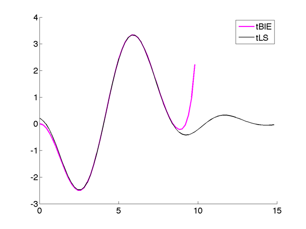
Note how the magenta line (computed using the boundary integral equation) diverges for |k|>8. However, the values of the magenta line for k near zero are very accurate.
Reconstruction from scattering transform using the D-bar method
Now we are ready to reconstruct the conductivity. Download the routines tBIErecon_comp.m and DB_oper.m, and run tBIErecon_comp.m.
You can look at the reconstruction using the routine recon_plot.m. You should see something like this:
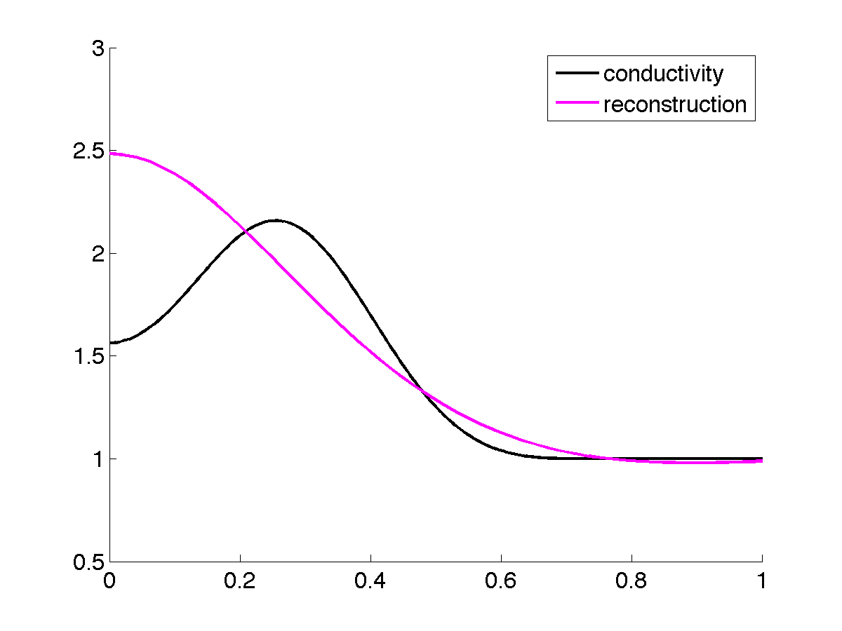
Here we used R=4, so the reconstruction is not very close to the original. Try setting M=8 and R=7 in tBIErecon_comp.m and see what recon_plot.m produces then.
Note carefully that although we used the rotational symmetry of the conductivity to speed up some of the above computations, the solution of the D-bar equation is a two-dimensional process, not one-dimensional. We did choose the reconstruction points along the positive x1-axis for convenience, but any planar point x could be chosen. Also, note that the reconstruction at one x point is completely independent from the reconstruction at another point, so the D-bar method allows region-of-interest imaging and trivial parallellization.
You can experiment with the truncation radius R. When you use tBIE computed using the boundary integral equation, you can take R up to 7 with no problems. However, when R is so large that the bad-quality parts of the above magenta plot are being used, the reconstruction will be bad.
You can take the experiment further by using tLS instead of tBIE; then you can push the reconstruction to higher values of R. Also, you can replace the low-quality tLS values near k=0 with the higher-quality tBIE.
![]()
