Hamilton-Jacobi Equations, Finite Differences, and Neural Networks

When designing an automatic device, an important aspect is ensuring that it runs as efficiently as possible. In optimal control theory, the goal is to determine a control policy that will drive a controlled dynamical system to maximize a performance criterion. This framework has ubiquitous applications ranging from aerospace trajectory planning and autonomous robotics to financial portfolio optimization and chemical process control.

The foundations of optimal control theory were forged in the intellectual heat of the Cold War, during which a geopolitical divide mirrored an interesting mathematical duality. In the U.S., Richard Bellman and Rufus Isaacs at the RAND Corporation were tackling the complexities of military logistics and aerial pursuit. They established the dynamic programming principle (DPP) [2], which focuses on the global value function that satisfies a Hamilton-Jacobi-Bellman equation — a perspective that naturally yields closed-loop feedback policies. By generalizing Bellman’s framework to differential games involving adversarial agents, Isaacs derived the Hamilton-Jacobi-Isaacs equation to solve zero-sum games in the 1960s. Simultaneously, Soviet mathematician L.S. Pontryagin and his school at the Steklov Institute addressed critical trajectory problems of the Space Race with Pontryagin’s maximum principle. This approach provided the necessary conditions for optimality, offering a powerful variational tool for characterizing specific optimal trajectories [3]. 

The value function \(u(x)\) of an optimal control problem provides a state-dependent feedback policy to optimally control the underlying system’s dynamics (described by \(f\)), minimizing the sum of the running cost \(r\) along the way:

\[\alpha_{*}(x) = \arg {\max}{_{\alpha}}\; \{ -f(x,\alpha) \cdot \nabla u(x) - r(x, \alpha)\}.\]

Under mild conditions on \(f\) and \(r\), the value function is differentiable almost everywhere and satisfies a Hamilton-Jacobi (HJ) equation at the points of differentiability together with a Dirichlet boundary condition determined by the terminal cost. For deterministic problems, HJ equations are first-order partial differential equations (PDEs) of the general form

\[H(x,\nabla u) = 0, \quad \text{in} \ \Omega \subset \mathbb{R}^n,\]

where \(H\) is the Hamiltonian function. The domain \(\Omega\) may include a time dimension as well.

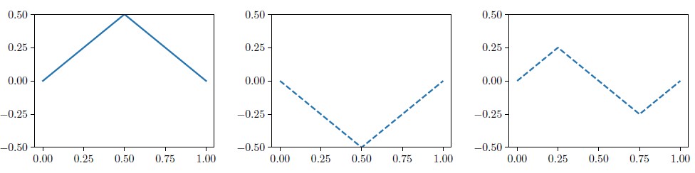
However, HJ equations are typically nonlinear PDEs, and classical \((C^1)\) solutions do not exist globally — even with smooth boundary data. Characteristic curves carry information from the boundary and thus inevitably intersect, leading to the formation of “kinks” or discontinuities in the gradient. In contrast, there are no unique continuous functions that satisfy the HJ equation at almost every point of the domain, along with the boundary condition. For example, the Eikonal equation \(|u_x| = 1\) on the interval \([0,1]\) with zero boundary condition \(u(0)=u(1)=0\) admits infinitely many such solutions (see Figure 1). Yet only one of these solutions corresponds to the value function of the optimal control problem for the shortest path to the boundary; this solution is represented in the left plot in Figure 1.

In the 1980s, Michael G. Crandall and Pierre-Louis Lions introduced the notion of the viscosity solution, providing a definitive existence and uniqueness theory [5]. The viscosity solution unequivocally selects the physically meaningful solution (i.e., the value function) from potentially infinite weak candidates. The name “viscosity solution” arises from the characterization of the solution by means of the vanishing viscosity method, which selects the unique solution by taking the limit as \(\varepsilon\to 0\) in the semilinear elliptic equation \(H(x, \nabla u_\epsilon)=\epsilon \Delta u_\epsilon.\) An analogous characterization of the viscosity solution regulates the solution’s behavior at its nondifferentiable kinks by testing the equation against smooth functions that touch the graph from above and below. In a typical case, including the one-dimensional (1D) Eikonal equation, the viscosity solution must be locally concave at any extremal point — a consequence of the vanishing viscosity limit.

Classical Numerical Methods

For decades, the standard approach to computing viscosity solutions has relied on fixed grids. In this framework, the computational domain \(\Omega\) is discretized into a Cartesian mesh, and the value function \(u(x)\) is approximated by a function that is defined on the grid nodes. To ensure convergence to the correct viscosity solution, one must rely on the theory of Guy Barles and Panagiotis E. Souganidis, which guarantees that any finite difference discretization that satisfies monotonicity, consistency, and stability will converge to the unique viscosity solution [1].

However, classical monotone schemes are often limited to low-order accuracy. To achieve higher-order accuracy while handling discontinuities (kinks) robustly, essentially non-oscillatory (ENO) and weighted ENO (WENO) methods that are built on top of monotone schemes have become standard tools in this domain.

Prominent algorithms for boundary value problems include the fast marching methods and fast sweeping methods. Crucially, these methods work because they strictly adhere to the DPP. In plain English, the DPP states that the optimal strategy from any point involves making the best immediate decision and then proceeding optimally from the resulting new state [2]. The results are essentially one- or finite-pass (through the grid) algorithms, where the grid acts as the medium through which the “optimality information” propagates. For time-dependent problems with explicit time integration, the evolution is naturally one-pass.

The Curse of Dimensionality

While highly efficient in low dimensions (i.e., from one to three dimensions), grid-based methods become infeasible in higher dimensions \(d\) due to the increasing number of grid nodes, which grow exponentially with \(d.\)

This explosion is not merely due to the need to maintain resolution for the fine properties of the solution. The fundamental issue is that to propagate the causality that the DPP requires, grid nodes must exist everywhere in the domain to accumulate the running cost from the boundary to the interior in an orderly fashion as dictated by the system’s characteristics. Even if the solution is primarily smooth and fine detail resolution is only necessary in a small region, the grid must still fill the entire ambient space to serve as the “conduit” for information flow. For a six-dimensional state space—a humble requirement for a modern robotic system—a modest grid of 100 points per dimension would require \(10^{12}\) nodes, rendering classical storage and computation intractable.

While representation formulas like Hopf-Lax or Cole-Hopf transformation exist for cases of HJ equations [6], and Riccati theory handles linear-quadratic cases, general nonlinear systems—especially those in robotics or games—require robust numerical approximations.

Residual Minimization and Neural Networks

To address these challenges, we turn to the representational power of artificial neural networks. The universality of deep neural networks ensures the efficient approximation of viscosity solutions to HJ equations, which—while lacking classical derivatives on the entire domain—are typically Lipschitz continuous. By parameterizing the solution with a neural network, we avoid grid dependencies and treat the solver as an optimization task, leveraging the computational infrastructure of gradient-based learning and graphics processing units.

It is tempting to formulate this optimization by minimizing the PDE residual, a strategy that has gained immense popularity through the development of physics-informed neural networks (PINNs) [8]. In this framework, one would typically define a loss functional such as

\[\mathcal{L}(u) = \int_\Omega H(x, \nabla u)^2 dx + \lambda \int_\Gamma (u(z) - g(z))^2 dz.\]

However, for HJ equations, this direct residual minimization approach is fundamentally ill-posed; as the 1D Eikonal equation in Figure 1 demonstrates, there are infinitely many Lipschitz-continuous functions that satisfy the equation almost everywhere. Thus, the loss function cannot distinguish the unique viscosity solution from these spurious candidates.

Without a mechanism to enforce the entropy-like selection criteria of Crandall and Lions, a neural network that minimizes \(\mathcal{L}(u)\) may easily converge to a “physically” incorrect, weak solution. To reliably recover the value function, one must find a way to embed the viscosity solution’s selection principles directly into the loss functional.

A Grid-based Method Without Grids

We advocate for an alternative path: rather than minimizing a continuous residual, we minimize a loss derived from a convergent finite difference approximation [7]. The numerical diffusion in a suitable finite-difference approximation regularizes the solution and enforces the selection of the viscosity solution. In a consistent and monotone finite difference method, the viscosity selection criteria are naturally satisfied by the discretization itself. In this framework, the neural network is trained to minimize a loss functional based on a numerical Hamiltonian \(\hat{H}\):

\[\mathcal{L}_h(u) = \int_{\Omega} |\hat{H}(x, \nabla_h u(x))|^2 \, dx + \lambda \int_{\Gamma} |u(z) - g(z)|^2 \, dz,\]

where \(\nabla_h\) denotes a discrete gradient operator that is evaluated using a stencil of size \(h.\) A particularly convenient choice is the Lax–Friedrichs discretization, where \(\hat{H}\) incorporates a controlled amount of numerical diffusion to stabilize the system. With the right amount of diffusion, one can ensure that gradient descent iterations applied to \(\mathcal{L}_{h}(u)\) converge to the unique global minimizer [7].

We can show that, for more general classes of monotone discretizations, gradient descent converges faster for larger values of \(h\) [2]. Additionally, training with larger values of \(h\) also tends to be more data efficient. So it is impractical to begin minimizing \(\mathcal{L}_h(u)\) with a very small \(h\).

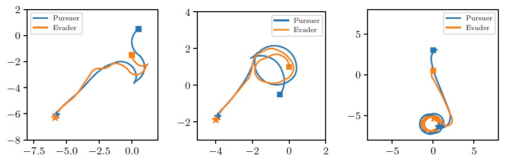
At the same time, we are interested in a sufficiently accurate finite-difference approximation of the viscosity solution. Crucially, one can employ a multilevel “warm-start” strategy. While the loss is defined using finite-difference stencils, the method remains grid-free. We do not solve a system on a fixed mesh; instead, we minimize the loss using stochastic gradient descent, in which we sample collocation points \(x\) across the domain and evaluate the finite difference \(\nabla_h\;u(x)\) on the fly. By first training the neural network with a larger \(h,\) we achieve faster initial convergence. Then, we progressively refine the discretization by decreasing \(h\) and continue the training to find a more accurate approximation of the viscosity solution. Training using this hierarchical approach typically requires only a few minutes on a standard laptop to compute high-fidelity value functions for some nontrivial model systems, such as the four-dimensional pursuit-evasion game for two Reeds-Shepp’s car models (see Figure 2).

Theory-informed Learning

Reflecting on these developments, we see that the success of neural network-based solvers for HJ equations relies on more than approximation power; it requires a deliberate connection to the underlying theory of viscosity solutions. While the standard residual-minimization approach is a powerful general framework, the specific non-uniqueness of HJ weak solutions necessitates a selection principle to recover the value function. By incorporating monotone discretizations directly into the loss functional, we bridge the convergence theory of classical numerical analysis with the scalability of modern deep learning.

This framework suggests a promising path forward for high-dimensional problems. Based on the mathematical foundations of Crandall-Lions and Barles-Souganidis, similar strategies should be applicable to viscous HJ equations in stochastic optimal control and other challenging fully nonlinear or degenerate elliptic operators. Ultimately, by using structural insights from numerical analysis to guide the optimization of neural networks, we can make complex, high-dimensional control tasks accessible on standard hardware — without the memory bottlenecks of the past.

References
[1] Barles, G., & Souganidis, P.E. (1991). Convergence of approximation schemes for fully nonlinear second order equations. Asymptot. Anal., 4(3), 271-283.
[2] Bellman, R. (1966). Dynamic programming. Science, 153(3731), 34-37.
[3] Bokanowski, O., Esteve-Yagüe, C., & Tsai, R. (2026). Solving Hamilton-Jacobi equations by minimizing residuals of monotone discretizations. Preprint, arXiv:2601.21764. 
[4] Boltyanskii, V.G., Gamkrelidze, R.V., & Pontryagin, L.S. (1960). Theory of optimal processes. I. The maximum principle. Izvestiya Rossiiskoi Akademii Nauk. Seriya Matematicheskaya, 24(1), 3-42.
[5] Crandall, M.G. & Lions, P.L. (1983). Viscosity solutions of Hamilton-Jacobi equations. Trans. Amer. Math. Soc., 277(1), 1-42.
[6] Darbon, J., & Osher, S. (2016). Algorithms for overcoming the curse of dimensionality for certain Hamilton–Jacobi equations arising in control theory and elsewhere. Res. Math. Sci., 3(1), 19.
[7] Esteve-Yagüe, C., Tsai, R., & Massucco, A. (2025). Finite-difference least square methods for solving Hamilton-Jacobi equations using neural networks. J. Comput. Phys., 524, 113721.
[8] Raissi, M., Perdikaris, P., & Karniadakis, G.E. (2019). Physics-informed neural networks: A deep learning framework for solving forward and inverse problems involving nonlinear partial differential equations. J. Comput. Phys. 378, 686-707.