Machine Learning for Dynamical Systems and Vice Versa: From Data Assimilation to Optimal Control

The topics discussed in this article about data assimilation (DA) and optimal control are unified by a common philosophy: leveraging machine learning (ML) for dynamical systems and, conversely, using system-theoretic insights to improve ML. ML offers new ways to overcome long-standing computational barriers, while dynamical systems theory provides analytical and computational tools that enhance the efficiency and reliability of learning. Our recent research sits precisely at this intersection of systems theory and ML [1].

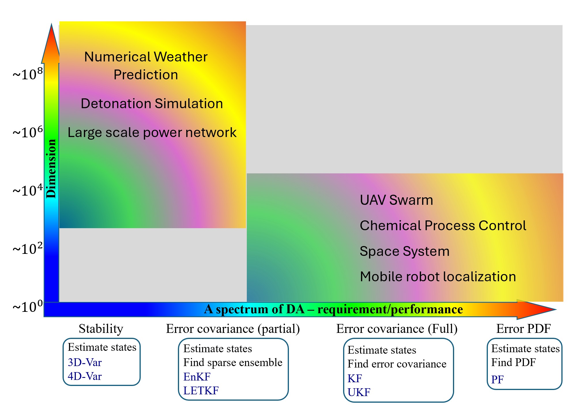
The primary goal of DA is to combine experimental observations with numerical models to obtain an optimal estimate of the system state, or its parameters, of a dynamical system. Current methods include variational approaches and sequential filters, but they are all impacted by the phenomenon known as the curse of dimensionality. For dynamical systems that arise from the discretization of partial differential equations (PDEs), the implementation cost of existing DA methods can easily exceed the memory and computational limits of modern computers. In general, algorithms that provide more detailed uncertainty information require significantly greater computational resources (see Figure 1). Many numerical models—such as those used in atmospheric dynamics and other large-scale engineering systems—have extremely high dimensions that make it infeasible to compute or represent full-error covariance information with conventional DA methods. Although the examples shown in Figure 1 do not represent an exhaustive list of applications, the colored regions illustrate the practical trade-off between model dimension and estimation capability. The upper-right corner of the diagram—where high dimensional systems intersect with the need to estimate full probability distributions—remains largely unexplored. These are precisely the types of problems where emerging artificial intelligence (AI)-based tools may lead to transformative advances.

A fundamental question in AI-based DA is: how much data is sufficient? When the data form a time sequence generated by an underlying dynamical system, this question is closely related to the ideas of observability and detectability, a classical concept in control theory. In [1], we refine this concept. For simplicity, consider the linear system

\[\begin{array}\mathbf{u}(k+1)=A\mathbf{u}(k), \mathbf{u}\in{\mathbb{R}}^n, k\in\mathbb{N}_0, \\\\ \mathbf{y}(k)=H\mathbf{u}(k)+\nu(k), \mathbf{y}\in\mathbb{R}^m, \\\\ z(k)=W\mathbf{u}(k), z\in\mathbb{R}, \end{array}\]

\(A\in\mathbb{R}^{n{\times}n}, \; W\in\mathbb{R}^{1{\times}n}, \; H\neq0\) and \(H\in{\mathbb{R}}^{{m}{\times}{n}},\) with \(z\) representing the quantity of interest (QoI). In classical control theory, the system is said to be observable if the initial state \(\mathbf{u}(0)\) can be uniquely determined from the sequence of observations \(\{\mathbf{y}(k)\}^K_{k=0}.\) We broaden this notion by introducing a quantitative measure of estimation uncertainty [1]. Specifically, define

\[\begin{array}{c}\rho^2=\underset{\{\hat{\mathbf{u}}(k)\}}{\textrm{max}}(W\hat{\mathbf{u}}(K)-z(K))^2,\\\\ \textrm{subject to}\quad\hat{\mathbf{u}}(k+1)=A\hat{\mathbf{u}}(k), \quad k=0,1,...,K-1, \\\\ \sum^{K}_{k=0}||H\mathbf{\hat{u}}(k)-H\mathbf{u}(k)||^2_2\leq{\epsilon}^2. \end{array}\]

The quantity \(\rho\) measures the worst-case estimation error over all trajectories whose dynamics and observation satisfy the constraints above. For this reason, we call \(\rho\) the ambiguity bound of the estimation problem. When using estimators that exploit additional information beyond the observation data, one may obtain estimates that outperform this worst-case bound. Nevertheless, it provides a fundamental benchmark: the error of a well-designed estimator should be smaller than \(\rho,\) as a smaller value of \(\rho\) typically indicates stronger observability of the quantity.

This definition generalizes the classical notion of observability. If the QoI \(z(K)\) is the initial state \(\mathbf{u}(0),\) then the ratio \({\epsilon}^2/{\rho}^2\) equals the smallest eigenvalue of the system’s observability Gramian. For nonlinear systems, the value of \(\rho\) can be approximated using empirical Gramians, which provides a practical way to assess the information content of observations.

In ML-based surrogate DA models, such as our approach developed in [1], a neural network is trained to learn the mapping from observations to the system state. Using a two-dimensional viscous Burgers equation as an example, we illustrate how the ambiguity bound can guide the design of such learning-based DA methods.

The ambiguity bound helps determine whether the observation sequence \(\mathbf{y}(k)\) within a given time window contains sufficient information about the QoI. Ideally, the value of \(\rho\) should be smaller than the desired estimation error tolerance; even a well-trained neural network is unlikely to produce accurate estimates if \(\rho\) is larger. In addition, for a QoI defined over a spatial region, \(D_{QoI},\) the ambiguity bound can be used to identify an effective region, denoted by \(D_{effective},\) that contains \(
D_{QoI}.\) Outside this region, the value of \(\rho\) becomes essentially constant; this indicates that the dynamics beyond \(D_{effective}\) have little or no influence on the estimation of the QoI. This observation enables a substantial reduction in computational cost. When training data is generated for the surrogate DA model, the numerical simulation can therefore be restricted to the effective region with an appropriate artificial boundary condition, thereby forming a reduced-order model that avoids solving the PDE over the entire domain.

We now turn to optimal control, where similar principles guide the integration of ML and dynamical systems. From autonomous vehicles to spacecraft maneuvering, modern engineering systems require controllers that operate reliably in complex and uncertain environments. Optimal control provides a systematic framework to design such control laws and plays a central role in a wide range of engineering applications.

A typical optimal control problem seeks a control input \(\pmb{u}(\cdot)\) that minimizes a performance metric subject to a dynamical system,

\[\left\{ \begin{array}{c}\underset{\mathbf{u}(\cdot)\in\mathbb{U}}{\textrm{minimize}} \; J[\pmb{u}(\cdot);{\pmb{x}_0}]=\mathcal{F}(\pmb{x}(t_f))+\int^{t_f}_{0}\mathcal{L}(t,\pmb{x},\pmb{u})dt,\\ \textrm{subject to}\quad \pmb{\dot{x}}(t)=f(t,\pmb{x},\pmb{u}), \quad\pmb{x}(0)=\pmb{x}_0.\end{array} \right.\]

For a given initial condition \(\pmb{x}_0\) the optimal trajectory and control \(\pmb{x}^*(t), \; \pmb{u}^*(t),\) must satisfy the necessary conditions of Pontryagin’s minimum principle, whose solutions produce an open-loop optimal control.

In many applications, however, it is desirable to design a feedback control law that depends on the current state of the system,  \(\pmb{u}(t, \pmb{x}(t)).\) This improves robustness to disturbances and modeling uncertainties and enables real-time implementation, hence the use of dynamic programming, whose central object is the value function \(V(t,\pmb{x}),\) which represents the minimum achievable cost starting from a given state. This function satisfies the Hamilton-Jacobi-Bellman (HJB) equation, a nonlinear PDE whose solution encodes the optimal feedback control through a Hamiltonian minimization condition. Despite its benefits, this approach is also subject to the curse of dimensionality, as it becomes intractable at high dimensions. As a result, classical optimal feedback control methods are limited to special cases such as linear quadratic regulators or low dimensional nonlinear systems.

Recent advances in ML offer new ways to address these challenges. Neural networks are remarkably effective at representing complex high-dimensional functions. It is now possible to use neural networks to approximate value functions or control policies and revisit optimal feedback design for high-dimensional nonlinear systems. These developments have led to growing interest in ML-based approaches to optimal feedback control, but they come with their own set of challenges. Applying neural networks to the HJB equation may admit multiple solutions, among which only the viscosity solution corresponds to the true value function. Consequently, minimizing the residual of the HJB equation at sampled points, as done in physics-informed neural networks, does not guarantee that the learned solution corresponds to the viscosity (and hence optimal) value function. A promising path forward is to incorporate structural insights from optimal control theory into the learning process, rather than rely purely on generic function approximation. 

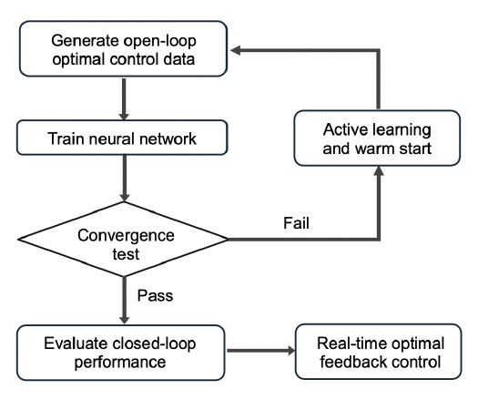
Although computing optimal feedback control is difficult for high-dimensional systems, many powerful algorithms exist for computing open-loop optimal solutions. These include indirect methods that solve the boundary value problems arising from Pontryagin’s minimum principle and direct methods that discretize the optimal control problem into a finite-dimensional optimization problem. Such techniques have been successfully applied to complex nonlinear systems. By repeatedly solving open-loop optimal control problems for randomly selected initial conditions \(\pmb{x},\) one can generate datasets that contain not only the optimal cost \(V^{(i)}\) but also the optimal trajectory \(\pmb{x}^{*^{(i)}}\), control \(\pmb{u}^{*^{(i)}}\) and costate variables \(\mathbf{\lambda}^{(i)}.\) These quantities provide rich and highly accurate information about the structure of the optimal solution and can be used to train and validate neural-network approximations of the value function and the associated feedback control.

Additionally, physics-informed training must be integrated. Rather than training neural networks solely to fit sampled values of the value function, the learning process can incorporate structural relationships from optimal control theory. For example, the training objective for a data set \(\mathcal{D},\) may combine multiple loss terms,

\[\mathcal{L}(\mathbf{\theta};\mathcal{D})=\textrm{loss}_V+{\mu}_{\lambda}\textrm{loss}_{\lambda}(\mathbf{\theta};\mathcal{D})+{\mu}_u\textrm{loss}_u(\mathbf{\theta};\mathcal{D}),\]

where \(\textrm{loss}_V\) is the mean squared error of value function and the additional loss terms—\(\textrm{loss}_{\lambda},\) based on costate data, and \(\textrm{loss}_{u},\) based on control data—enforce relationships derived from optimal control theory. In particular, the costate variable is the gradient of the value function, and the optimal control is determined from the value function through the Hamiltonian minimization condition, thus significantly improving training efficiency and accuracy.

Control-theoretic insights can also guide the design of neural network feedback architectures. Although neural networks can achieve high training accuracy, controllers obtained purely from data may fail to stabilize the system when deployed in closed-loop operation. Recent work addresses this with classical optimal control designs such as the linear quadratic regulator. These hybrid architectures combine the reliability of classical control with the expressive power of deep learning. To further enhance both efficiency and reliability, components can be integrated into an adaptive learning framework (see). In this scheme, an initial controller trained on a limited dataset generates approximate closed loop trajectories and costates, which serve as effective initial guesses to warm-start open-loop optimal control solvers. This significantly improves convergence and computational efficiency of the open-loop solvers. Moreover, it enables targeted data acquisition, particularly in regions where the current controller underperforms. Through this iterative, performance-driven process, the controller is progressively refined toward accurate and efficient optimal feedback control. 

These ideas have been tested on several high-dimensional control problems, from spacecraft attitude control to systems of PDEs [2] and nonlinear unmanned aerial vehicles [3]. Together, recent developments point toward a new paradigm in which data, models, and control are tightly integrated through learning. By combining theoretical insights from dynamical systems with the expressive power of neural networks, researchers can address problems once deemed intractable. Continued progress along this direction may significantly expand the scope and impact of DA and optimal control in science 
and engineering.

Wei Kang delivered a plenary talk on this topic, titled “Deep Learning Meets System Theory: A Collaborative Frontier in Control Engineering and Data Science,” at the 2025 SIAM Conference on Control and Its Applications (CT25), which took place last July in Montréal, Québec, Canada. Kang, Qi Gong, and Lars Grüne also delivered a two-session minisymposium on this topic at CT25.

References   
[1] Kang, W., Xu, L., & Zhou, H. (2024). Observability and effective region of partial differential equations with application to data assimilation. SIAM J. Sci. Comput., 46(3), 249-271.
[2] Nakamura-Zimmerer, T., Gong, Q., & Kang, W. (2021). Adaptive deep learning for high dimensional Hamilton-Jacobi-Bellman equations. SIAM J. Sci. Comput., 43(2), A1221-A1247.
[3] Nakamura-Zimmerer, T., Gong, Q., & Kang, W. (2022). Neural network optimal feedback control with guaranteed local stability. IEEE Open J. Control Syst., 1, 210-222.